Chapter 46 — Links Between Macroeconomic Problems and Their Interrelatedness
Cambridge International AS & A Level Economics (9708) · Unit 10.2 · 4th edition coursebook
Learning objectives
- Describe the relationship between the internal value of money and the external value of money.
- Explain the relationship between the balance of payments and inflation.
- Explain the relationship between growth and inflation.
- Explain the relationship between growth and the balance of payments.
- Explain the relationship between inflation and unemployment.
- Analyse the traditional Phillips curve.
- Analyse the expectations-augmented Phillips curve (short- and long-run Phillips curve).
Key terms
- Phillips curve
- a curve that shows the relationship between the unemployment rate and the inflation rate over a period of time.
- expectations-augmented Phillips curve
- a diagram that shows that while there may be a trade-off between unemployment and inflation in the short run there is no trade-off in the long run.
46.1The relationship between the internal and external value of money
The internal value of a country's currency is the purchasing power of one unit of that currency in the domestic market — what a dollar, a pound or a peso buys at home. The external value is the rate at which it exchanges for other currencies. The two values are linked. Inflation reduces internal value: each unit of the currency buys less than before.
If a country's inflation rate rises above that of its rival countries, foreigners demand fewer of its now-more-expensive exports, so demand for the currency on the foreign exchange market falls. At the same time, domestic households and firms switch to relatively cheaper imports, so the supply of the currency on the foreign exchange market rises. Lower demand and higher supply combine to depreciate the currency (see Figure 46.3).
The link runs in the other direction too. A fall in the exchange rate raises the home-currency price of imports. Each unit of the currency now buys fewer of the now more expensive imported goods, so the internal value falls. The example often used is a bilateral exchange rate moving from US$1 = 8 Argentine pesos to US$1 = 6 Argentine pesos: an Argentine import priced at 480 pesos rises from US$60 to US$80 once converted. Purchasing power is also eroded indirectly. The rise in the price of imported raw materials pushes up domestic costs, and the reduction in competitive pressure from imports allows domestic firms to lift their own prices. So internal and external values of a country's money tend to move directly together: a fall in the internal value leads to a fall in the external value and vice versa.
This relationship is the most common case but it is not automatic. A country may experience domestic inflation yet still see its external value rise — for example, if it operates a fixed exchange rate, or if its inflation rate is still below that of its rival trading partners.
46.2The relationship between the balance of payments and inflation
If a country's inflation rate rises above that of its main competitors, its price competitiveness falls. Export revenue declines, import expenditure rises, and the current account balance deteriorates. The causation also runs the other way: an increase in the current account surplus can itself cause inflation, because net exports are making an increasing contribution to aggregate demand and more money is flowing into the country than is leaving it.
That upward pressure on the domestic price level — and the matching downward pressure on the internal value of the currency — may be short-lived. An increasing current account surplus tends to cause an appreciation of the exchange rate. The stronger currency in turn reduces the surplus and lowers the inflation rate, because the price of imported products falls and domestic firms come under more pressure to keep their own prices low.
The financial account can also affect inflation. A net inflow on the financial account — for example, foreign direct investment by multinational companies — may reduce inflation if those firms bring in advanced technology and add to competitive pressure inside the economy.
Key concept link — Time
The effect of economic growth on the current account of the balance of payments may vary in the short run and long run.
46.3The relationship between growth and inflation
A high rate of inflation is likely to reduce a country's economic growth rate. Higher domestic prices erode price competitiveness, so net exports fall, lowering aggregate demand. Reduced aggregate demand reduces output — or at least slows the growth of output.
The effect running the other way is less clear-cut. Actual economic growth may be accompanied by either cost-push or demand-pull inflation. As more is produced, firms compete more aggressively for resources, including labour, so input prices and wages rise. The extra output also generates extra income, which feeds back into aggregate demand. The gap between rising aggregate demand and the economy's ability to expand output gets more acute as the economy approaches full employment, so the inflationary pressure intensifies.
Potential economic growth — growth in productive capacity — can reduce inflation rather than add to it. It allows aggregate demand to expand without pushing the price level up, and it can directly reduce unit costs of production. Advances in technology, for example, let a higher output be produced per factor input, lowering the cost of each unit.
Key concept link — Equilibrium and disequilibrium
A change in a country's inflation rate can cause a change in the equilibrium level of national income.
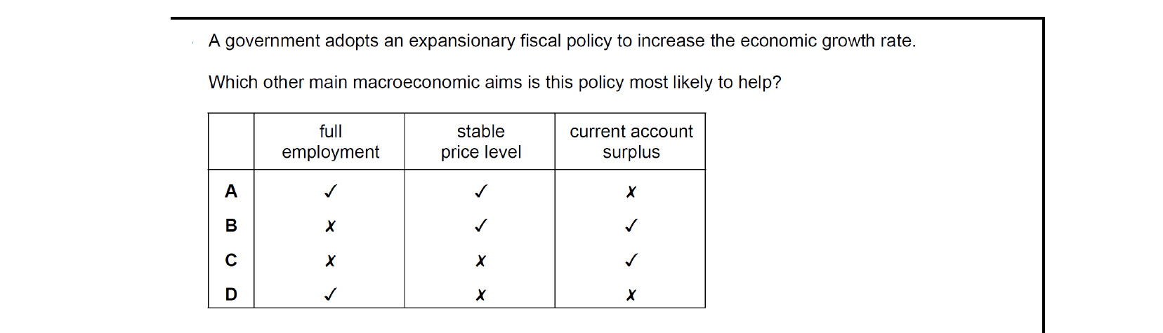
Expansionary fiscal policy raises aggregate demand, lifting output and employment — so full employment is helped. But the same demand expansion pulls up the price level (worsening stability) and sucks in extra imports, hurting any current-account surplus. The aim it directly assists is full employment alone, not price stability or a current-account surplus.
46.4The relationship between growth and the balance of payments
Economic growth can be export-led: a rise in net exports raises GDP by a multiple amount through the multiplier effect, and the same change improves the current account. Potential economic growth can produce a similar positive relationship, because expanding capacity tends to raise the price competitiveness — and, depending on what is being expanded, the quality competitiveness — of the country's products.
The relationship can also be inverse, at least in the short run. To produce a higher output, firms may import more raw materials and capital goods. If part of the resulting extra output is then exported, the initial rise in imports may eventually be matched by a rise in exports, but the timing of the two flows is not the same.
Causation can run from the balance of payments to growth as well as the other way around. An increase in a current account surplus raises aggregate demand, which can stimulate actual economic growth.
46.5The relationship between inflation and unemployment
The relationship between inflation and unemployment has been one of the most heavily studied questions in macroeconomics. Economists have looked at how changes in inflation can affect unemployment, how changes in unemployment can affect inflation, and how government policies aimed at reducing unemployment end up influencing both variables together.
The Phillips curve
The most famous study was published in 1958 by Bill Phillips, a New Zealand economist based at the London School of Economics. He analysed historical data on unemployment and money wages — used as an indicator of inflation — in the UK over the period 1861 to 1957, and found an inverse relationship between the two. The Phillips curve that summarised his finding slopes downward from left to right (see Figure 46.5).
The curve is not a straight line. It is steeper at low rates of unemployment, indicating that pushing unemployment from a very low rate to an even lower rate causes a sharp rise in inflation. As unemployment increases, the curve becomes much flatter, so further reductions in unemployment from a high base do less to raise inflation, and at very high rates of unemployment the economy may even experience deflation. The economic logic is that a fall in unemployment raises aggregate demand and puts upward pressure on wages, so the price level rises with it.
The traditional Phillips curve also implied that a government could choose its preferred combination of unemployment and inflation by moving along the curve. Faced with, for example, 8% unemployment and 4% inflation, a government could use expansionary fiscal or monetary policy to lower unemployment to 5%, accepting that the gain in employment would be bought at the cost of higher inflation.
The whole curve can shift. It shifts to the right if the inflation rate associated with any given unemployment rate increases — for example, if workers hold out for higher wages because they expect future inflation to be higher, or if workers become less skilled. Improvements on the supply side of the economy shift the curve to the left.
The expectations-augmented Phillips curve
The traditional Phillips curve is supported by Keynesians but is questioned by monetarists. Monetarists argue that, while there may be a short-run trade-off, in the long run policy tools that raise aggregate demand have no impact on unemployment and only succeed in raising the inflation rate. To support this view, the US economist Milton Friedman developed the expectations-augmented Phillips curve, drawn as a vertical line whose position is determined by the natural rate of unemployment (see Figure 46.6).
The story the diagram tells works like this. Suppose unemployment starts at 8% with low inflation. An increase in aggregate demand succeeds in pulling unemployment down to 4%, but it also pushes inflation up to 5%, moving the economy on to a higher short-run Phillips curve. Firms expand their output, and more people are drawn into the labour force by the higher wages on offer. Eventually firms realise that their own costs have risen in step, so their real profits are unchanged, and they cut output back. Some workers, recognising that real wages have not actually risen, leave the labour force. Unemployment returns to 8% in the long run, but 5% inflation has now been built into expectations: firms and workers assume inflation will continue at 5% when setting prices and wages. A second attempt to push unemployment down to 4% therefore moves the economy on to an even higher short-run Phillips curve, pushing inflation up to 12%, with the long-run unemployment rate still anchored at the natural rate.

The Phillips curve plots the trade-off between unemployment and inflation, with the unemployment rate on the horizontal axis and the inflation rate (the percentage change in the general price level) on the vertical axis. It is not real wages, take-home pay or the rate of interest that goes on the vertical axis — it is the rate of inflation.
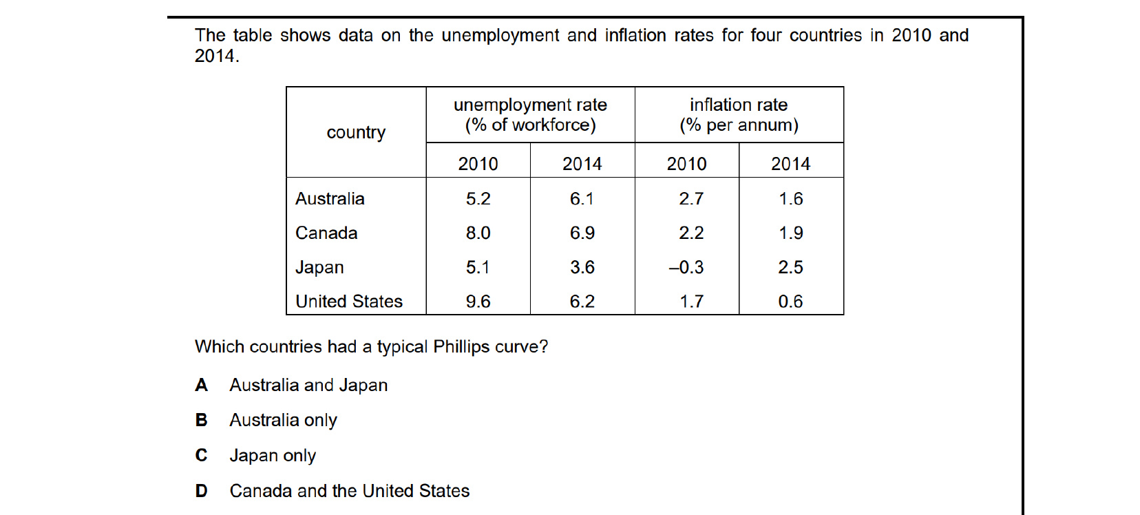
A typical Phillips curve shows an inverse relationship: when unemployment falls, inflation should rise (and vice-versa). Comparing 2010 and 2015: Australia's unemployment rose from 5.2 to 6.1 while inflation fell from 2.7 to 1.6 — inverse, consistent. Japan's unemployment fell from 5.1 to 3.6 while inflation rose from -0.3 to 2.5 — also inverse. Canada and the US show unemployment AND inflation both falling. So only Australia and Japan fit the typical curve.
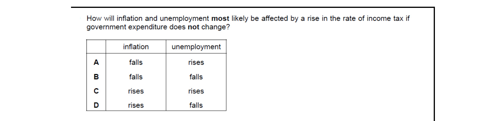
A higher rate of income tax reduces disposable income, so consumption and aggregate demand fall. Weaker demand eases price pressure, so inflation falls. But weaker demand for goods and services also reduces firms' derived demand for labour, so unemployment rises. Hence the pairing is falling inflation alongside rising unemployment.
End-of-chapter practice
Past-paper questions from CIE 9708. Pick A, B, C or D. Answers are saved on this device — press Download report (PDF) at the top to save them.
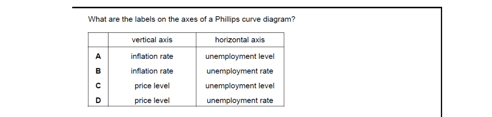
A Phillips curve diagram plots two rates: the rate of inflation (percentage change in the price level) on the vertical axis and the unemployment rate (percentage of the workforce out of work) on the horizontal axis. Levels of the price index or counts of unemployed workers are not used — both variables are expressed as rates.
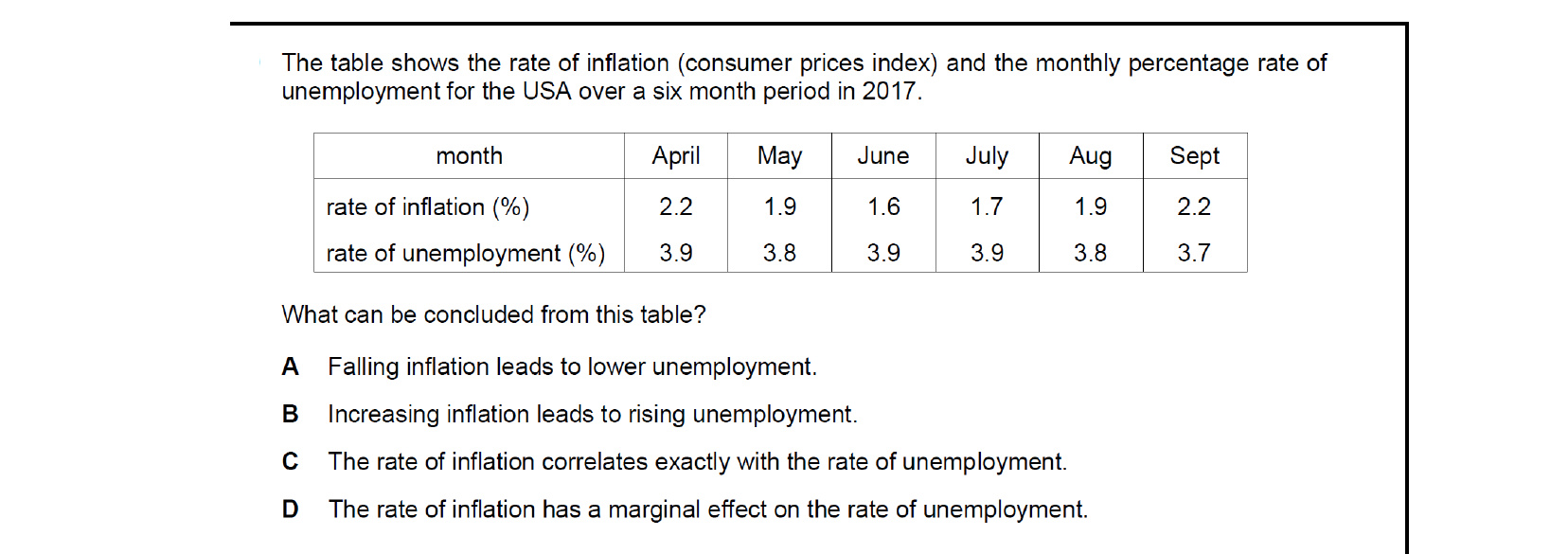
Over the six months, the inflation rate moves while the unemployment rate barely shifts (only between 3.7 and 3.9). With virtually no co-movement in unemployment, we cannot say falling inflation lowers unemployment, that rising inflation raises it, or that the two move exactly together. The only safe conclusion is that, over this short period, inflation has had only a marginal effect on unemployment.
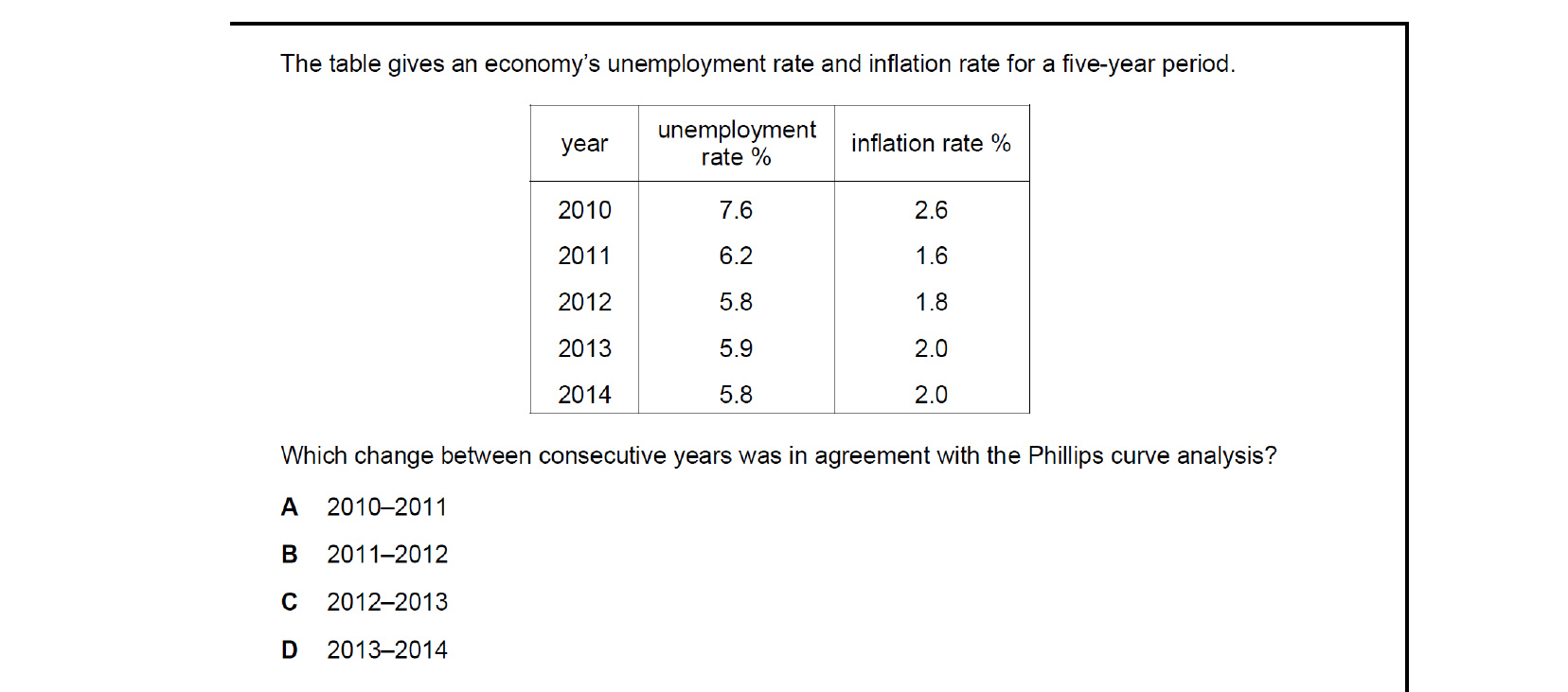
Phillips-curve analysis requires inflation and unemployment to move in opposite directions. Between 2010 and 2011 unemployment fell from 7.6 to 6.2 and inflation also fell — not consistent. Between 2011 and 2012 unemployment fell from 6.2 to 5.8 while inflation rose from 1.6 to 1.8 — an inverse relationship, exactly as the Phillips curve predicts. So the year-pair that fits is 2011–2012.
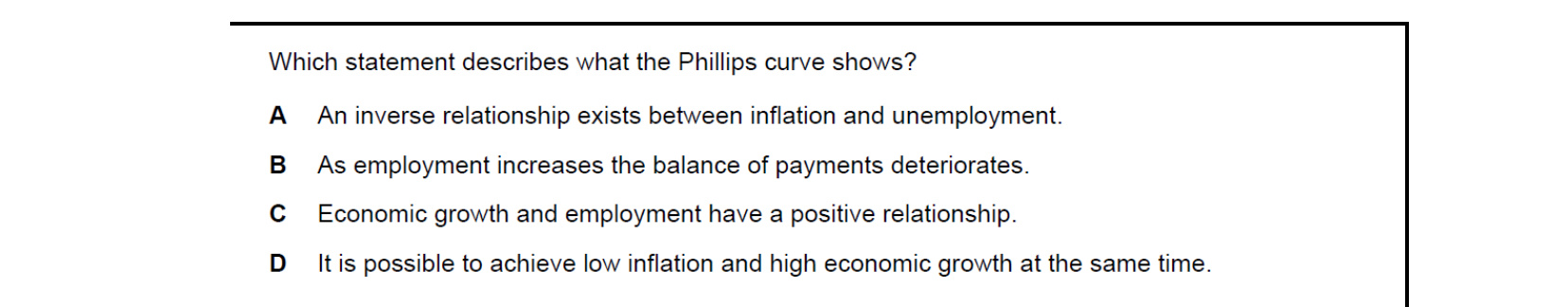
The Phillips curve plots the relationship between unemployment and inflation and historically shows that, in the short run, they tend to move in opposite directions: when unemployment falls, inflation rises, and vice versa. So the statement that captures the curve is that an inverse relationship exists between inflation and unemployment.

The vertical axis of the Phillips curve measures the rate of inflation — the percentage change in the general price level over a year — plotted against the unemployment rate on the horizontal axis. It does not measure real wages, take-home pay or the rate of interest; the curve's central message is the inflation–unemployment trade-off.
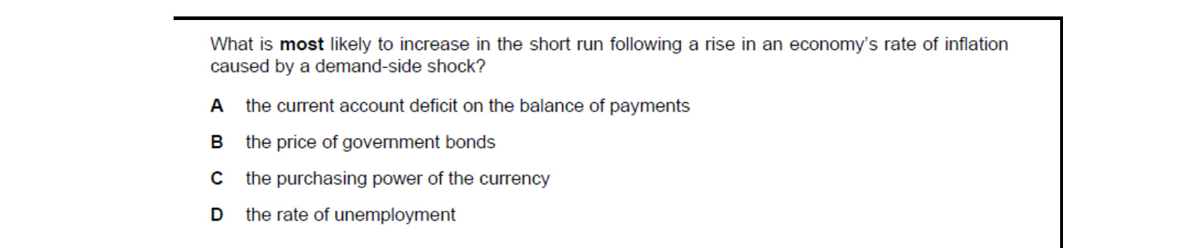
A demand-side shock pushing up inflation also pulls up imports as households spend more, while domestic goods become relatively dearer for foreign buyers. Both effects worsen net exports, widening the current account deficit. Higher inflation lowers (not raises) the purchasing power of the currency, depresses bond prices (yields rise), and tends to cut unemployment in the short run — so the deficit is what rises.
Attempt the practice questions above to build your score.
Self-evaluation checklist
After studying this chapter, you should be able to:
- Describe the relationship between the internal value of a country's currency and its external value.
- Explain the relationship between the balance of payments and inflation.
- Explain the relationship between growth and inflation.
- Explain the relationship between growth and the balance of payments.
- Explain the relationship between inflation and unemployment.
- Analyse the traditional Phillips curve (downward sloping from left to right) that suggests that government can reduce the unemployment rate at a cost of a higher inflation rate.
- Analyse the expectations-augmented Phillips curve (a vertical line) that suggests there is no long-run trade-off between unemployment and inflation.
Want more practice? Drill this chapter's past-paper MCQs (36 questions) →